Part 2: The basic operations of image processing
In the previous notebook, we've seen how to load and edit an image using Python. Let us now present the fundamental operations on which relies every single imaging software:
- truncation,
- subsampling,
- pixelwise mathematics,
- masking and thresholding,
- filtering (also known as convolution product).
But first, we need to re-import the necessary modules:
%matplotlib inline
import center_images             # Center our images
import matplotlib.pyplot as plt  # Graphical display
import numpy as np               # Numerical computations
from imageio import imread       # Load .png and .jpg images
We re-define our custom display routine:
def display(im):  # Define a new Python routine
    """
    Displays an image using the methods of the 'matplotlib' library.
    """
    plt.figure(figsize=(8,8))                    # Create a square blackboard
    plt.imshow(im, cmap="gray", vmin=0, vmax=1)  # Display 'im' using gray colors,
                                                 #     from 0 (black) to 1 (white)
And import an axial slice:
I = imread("data/aortes/1.jpg", as_gray=True)  # Import a jpeg image as grayscale array
I = I / 255  # For convenience, we normalize the intensities in the [0,1] range
display(I)   # Let's display our slice:

Truncation
To truncate (or crop) an image, we simply need to use the "range" syntax presented in the first notebook:
J = I[200:400, 100:300] # Restrict ourselves to a sub-domain of I
display(J)

Subsampling
Likewise, subsampling can be performed using the stepsize argument:
J = I[::2, ::2] # Only keep "one pixel in two" in both dimensions
display(J)

J = I[::8, ::8] # Only keep "one pixel in eight" in both dimensions
display(J)

Pixel-wise algebraic operations
Python is math-friendly: arbitrary operations can be performed on the variable I and are applied pixel-wise.
J = I / 2  # Halve the intensity across the full image
display(J)

J = 2 * I  # Double the intensity - we may saturate in the brighter regions
display(J)

J = I**2   # "Square" function, which darkens the grey pixels
display(J)

J = np.sqrt(I)  # "Square root", which brightens the grey pixels
display(J)

J = ((I**2) + np.sqrt(I)) / 2  # Arithmetic mean of the two previous images
display(J)

Masking, thresholding
More interestingly, Python also supports binary tests (which produce masks) and conditional indexing:
J = I > .5  # J = 0 or 1, depending on the dark/bright-ness of the current pixel in I
display(J)

J = I.copy()     # Copy the original image...
J[ J < .4 ] = 0  # And paint in black the darker pixels (intensity < .4)
display(J)

Filtering, convolutions
Finally, we present the building block of all texture-processing and feature-detection programs: the convolution - which is mathematical jargon for "local, weighted means across an image", i.e. what you get when you replace a pixel's value by a weighted average of its neighbours.
Such an operation can be implemented using truncations, multiplications and sums:
I_l = I[:,:-1]  # Select the full image, bar the last column
I_r = I[:, 1:]  # Select the full image, bar the first column

print(I.shape, I_l.shape, I_r.shape)  # I_l and I_r are slightly smaller than I
Here, we know that
for all indices i (row) and j (column).
Computing the halved sum of I_r and I_l is thus equivalent to super-imposing shifted versions of the raw image I, and allows us to compute efficiently an image J such that
J = .5* I_l + .5* I_r  # Weighted sum of I_r and I_l
display(J)

This operation only blurs the signal a little bit, and does not produce any spectacular effect.
However, by computing the difference I_r - I_l, we remark a key-feature of weighted sums: used with the correct weights (in this case, +1 and -1), they may allow us to detect edges. This is because if
then our filtered image J contains local differences of intensities between pixels and their neighbours to the right: a quantity that resembles an "x-derivative"
\begin{align} \frac{\partial I(x,y)}{\partial x}~\simeq~ \frac{I(x+1,y) - I(x,y)}{(x+1)-x} \end{align}
and is equal to zero if and only if I is locally constant in the horizontal direction.
J = I_r - I_l  # Difference between I_r and I_l

plt.figure(figsize=(8,8))                       # Square blackboard
plt.imshow( J, cmap="gray", vmin=-.5, vmax=.5); # Displays the image J in grayscale,
                                                #    from -.5 (black) to +.5 (white)

Most interestingly, I_r - I_l is nearly zero (= grey-ish in the plot above) in the constant regions of the image I, where I_r[i,j] = I[i,j+1] is nearly equal to I_l[i,j] = I[i,j].
This allows us to detect sharp transitions, which stand out on a mostly dull background.
To let us build upon this idea, the scipy library provides a correlate function which allows us to specify our weights as a "box image" (a convolution kernel) which slides along the image:
from scipy.ndimage import correlate

k = np.array([      # "Convolution kernel" = Small image = collection of weights
    [-1.,1.]        # -1 for the left shift "I_l", +1 for the right shift "I_r"
])                  # ==> Horizontal derivative

J = correlate(I,k)  # Computes the 'correlation' (= filtering, convolution)
                    # between the image 'I' and the kernel 'k'

plt.figure(figsize=(8,8))                       # Square blackboard
plt.imshow( J, cmap="gray", vmin=-.5, vmax=.5); # Displays the image J in grayscale,
                                                #    from -.5 (black) to +.5 (white)

k = np.array([      # "Convolution kernel" = Small image = collection of weights
    [1,1,1,1,1],
    [1,1,1,1,1],
    [1,1,1,1,1],    # Uniform weights on a 5x5 square
    [1,1,1,1,1],
    [1,1,1,1,1],
]) / 25             # ==> Weighted average on a small neighborhood, "blurring" effect

J = correlate(I,k)  # Computes the 'correlation' (= filtering, convolution)
                    # between the image 'I' and the kernel 'k'

display(J)

k = np.array([ # "Convolution kernel" = Small image = collection of weights
    [+1],      # +1 on top
    [-1],      # -1 on the bottom
])             # ==> Vertical derivative

J = correlate(I,k)  # Computes the 'correlation' (= filtering, convolution)
                    # between the image 'I' and the kernel 'k'

plt.figure(figsize=(8,8))                       # Square blackboard
plt.imshow( J, cmap="gray", vmin=-.5, vmax=.5); # Displays the image J in grayscale,
                                                #    from -.5 (black) to +.5 (white)

Exercise : Using the tools presented above, please implement an "edge detector", an image which is equal to 1 on edges (= sharp transitions) and zero elsewhere.
# À vous de jouer !
# =================
J = I # etc.

# =================
display(J)
Solution :
k_x = np.array([ # "Convolution kernel" = Small image = collection of weights
    [0, 0, 0],   #                                      in a 3x3 neighborhood
    [0,-1, 1],   # -1 center, +1 to the right
    [0, 0, 0],
])               # ==> Horizontal derivative

k_y = np.array([ # "Convolution kernel" = Small image = collection of weights
    [0,+1, 0],   # +1 top                               in a 3x3 neighborhood
    [0,-1, 0],   # -1 center
    [0, 0, 0],
])               # ==> Vertical derivative

I_x = correlate(I,k_x)  # x-derivative, detects vertical edges
I_y = correlate(I,k_y)  # y-derivative, detects horizontal edges

J = I_x**2 + I_y**2     # (positive) squared norm of the gradient
edges = J > .03         # We highlight pixels where the derivative is strong enough


display(I) ; plt.title("Input image 'I'")        # Input slice

# Fancy display: 'I_x' and 'I_y' side-by-side ---------------------------------------
plt.figure(figsize=(12,6))                       # Create a rectangular blackboard
plt.subplot(1,2,1)                               # (1,2) waffle, first cell
plt.imshow(I_x, cmap="gray", vmin=-.5, vmax=.5)  # Display I_x
plt.title("Vertical edges 'I_x'")                # Put a legend
plt.subplot(1,2,2)                               # (1,2) waffle, second cell
plt.imshow(I_y, cmap="gray", vmin=-.5, vmax=.5)  # Display I_y
plt.title("Horizontal edges 'I_y'")              # Put a legend

display(edges) ; plt.title("Final result") ;     # Display our final result


To remember: There is no magic. On "bitmap" images, which are nothing but numerical arrays, computer programs tend to rely on simple (and thus, cheap!) operations that can be computed fast on parallel hardware.
Most interestingly, convolutions allow us to implement feature detectors: using clever weights, we were able to turn a raw image into a meaningful semantic feature map. To follow the current trend, we can display the edge detector above as a simple convolutional neural network:
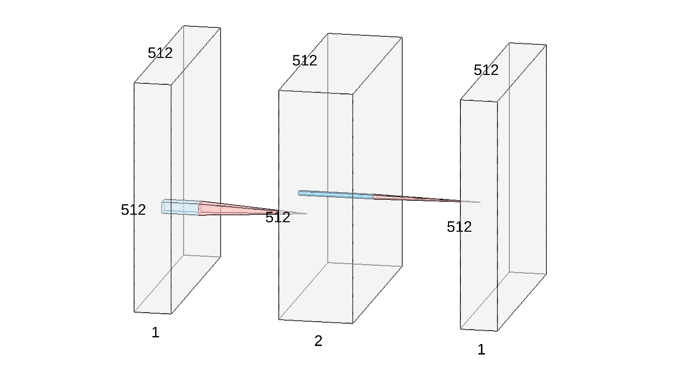
- On the left, you recognize our input 512x512 image
I. - In the middle, we represented the two intermediate feature maps
I_xandI_yas a stacked (2,512,512) volume. The red-and-blue transition indicates that these two images were computed fromIusing small, 3x3 convolution filters. - Finally, the output
edgesof our detector is represented by the rightmost image. It is computed from the previous block using a pointwise non-linearity: the squaring operation, followed by a sum and a thresholding.
Modern research on segmentation, texture analysis and feature detection is all about finding the correct weights for our 3x3 convolution filters (k_x, k_y, etc.). As we'll see in Part 7, mathematical theorems can be used in specific situations (e.g. for the JPEG2000 compression standard, which is ubiquitous in cinemas).
Convolutional Neural Networks. For medical applications, as of today, the preferred method is to use a simple optimization algorithm that fits a set of parameters (the weights) to a dataset, exactly as you do when you perform Linear Regression. Researchers and marketing people love to describe this approach as "biologically inspired", re-branding their work as "AI" and "neural networks"... But don't be fooled by this high-flown terminology: under the hood, most products work just like the python code presented above.